Quantum Transform’s Bimodal Distribution is analogous to the Schrodinger equation and is equal to the complex sum of the energy’s and order’s logarithmic distributions, where RLognormal[(Δf)h] is the real part and RLognormal(O) is the imaginary part.
Written below we get the eqation for the Quantum Information Field Energy randomness observed at the multibifurcation point of the spacetime:
Time crystal oscillator conceptual framework
The randomness observed in the Quantum Information Field Energy at the multidimensional bifurcation point in spacetime can be mathematically characterized by:
Eq. 1 Doktor Habdank’s formula
- H: Hamiltonian at point B
- RLognormal(∆E): Random log-normal distribution of energy changes
- j: Imaginary unit
- φ(t): Normal distribution expressed in Kelvins
- RLognormal(O): Random log-normal distribution of order
This equation describes the Hamiltonian’s operation at a specific point B on the state |Ψ(t)⟩, resulting in a change in the system’s energy (∆E), which follows a log-normal distribution. This variability is attributed to quantum fluctuations.
Eq.2 Wave function is a two component object (ѱ1 ,ѱ2 ), which can be written as a complex number ѱ = ѱ1 + iѱ2 , whose absolute square, |ѱ|2 = ѱ12 + ѱ22
Eq.3 represents the time-frequency uncertainty relation, derived from the more general Heisenberg Uncertainty Principle, while Eq.4 presents a stricter formulation of this uncertainty, imposing limits on our ability to simultaneously determine the frequency and duration of an event. These equations correspond to the initial trajectories following the BiQuantum Realm State point.
In quantum mechanics, energy (E) and frequency (f) are interrelated by the Planck relation: E = h ∙ f, where h denotes Planck’s constant.
Eq. 6 provides the probability of the i-th element among all elements.
Eq. 7 defines equation for a nonlinear oscillator, where:
- R1, R2: Random elements 1 and 2
- C1, C2: Capacitative elements 1 and 2
- I: Field
- U: Field’s Potential
Eq. 8 offers a generalized equation for nonlinear oscillator incorporating 26 random (RN) and capacitative (CN) elements.
Heisenberg uncertainty: frequency version which describes transition between the Minkowski space to tachyon space, where Δf is the frequency uncertainty and Δt is time uncertainty.
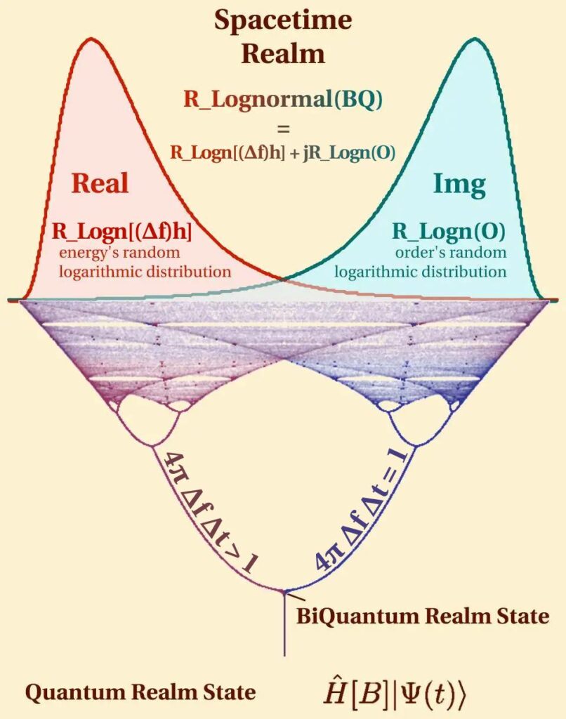
Bifurcation with asymmetry emerges from the Quantum Energy randomness with BiQuantum Realm State, where Quantum Transform’s Bimodal Distribution is equal to the complex sum, the real part RLognormal[(Δf)h] is random logarithmic distribution representing changes in system’s frequency uncertainty, while the imaginary part RLognormal(O) is order’s random logarithmic distribution. 4π Δf Δt = 1 and 4π Δf Δt > 1 describe transition between the Minkowski space to tachyon space, where Δf is the frequency uncertainty and Δt is time uncertainty [3].