Quantum Holo Glossary

Doktor Habdank

The Function-Gradient Quantum Gravity’s Potential State Theorem

The Function-Gradient Quantum Gravity’s Potential State Theorem proposes that the quantum state of any physical system in a gravitational field can be described by a wave function that depends on the potential state, the gradient force, and the gravitational field strength. This theorem aims to unify quantum mechanics and general relativity and may have implications for our understanding of the quantum properties of particles in gravitational systems and for the development of future quantum technologies.

Schrödinger's wave function equation

Hamiltonian (quantum mechanics) & Quantization of the electromagnetic field
In quantum mechanics, the Hamiltonian of a system is an operator corresponding to the total energy of that system, including both kinetic energy and potential energy. Its spectrum, the system’s energy spectrum or its set of energy eigenvalues, is the set of possible outcomes obtainable from a measurement of the system’s total energy. Due to its close relation to the energy spectrum and time-evolution of a system, it is of fundamental importance in most formulations of quantum theory.

The level spacings of GOE follow Wigner-Dyson distribution. As a comparison, a Poisson distribution is plotted as well. (Source: H. Nakayama)

Level spacing distribution follows Poisson or Wigner-Dyson distribution, indicates that they have found a signature for a
quantum integrable or chaotic system respectively. 

Hiroki Nakayama, “Random Matrix Theory, Quantum Chaos, and Eigenstate Thermalization“, July 2, 2020

BiQuantum Hamiltonian distribution

Quantum Transform’s Bimodal Distribution is analogous to the Schrodinger equation and is equal to the complex sum of the energy’s and order’s logarithmic distributions, where RLognormal(ΔE) is the real part and RLognormal(O) is the imaginary part.’

Written below we get the eqation for the Quantum Information Field Energy randomness observed at the multibifurcation point of the spacetime:

\hat {H}[B]|\Psi (t)\rangle => RLognormal(\Delta E) + j \frac{\varphi(t)}{RLognormal(O)}

Doktor Habdank’s formula

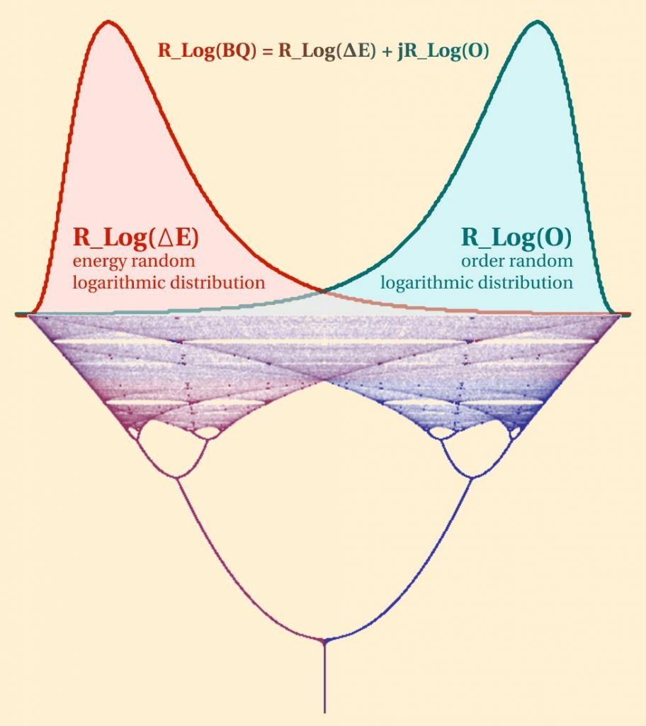
Tachyonic fields multibifurcation at the light speed 

Luxons, in the special relativity, are the massless particles with the invariant light speed [1] and thus they are the multibifurcation points for the tachyonic field. Beyond light speed, exist superluminal tachyon multibifurcation vibrators. Exciton-polariton X-waves are the superluminal wave equivalent [2] 

[1] Chashchina, Silagadze, BREAKING THE LIGHT SPEED BARRIER, ACTA PHYSICA POLONICA B, 2012

[2] Antonio Gianfrate, et al., Superluminal X-waves in a polariton quantum fluid, nature, 2017

Graph of |\psi_{100}|^2, with the classical distribution (dashed curve) superimposed

In the classical case we are talking about the distribution of positions over time for one oscillator, whereas in the quantum case we are talking about the distribution over an ensemble of identically prepared systems.

Source https://www.physicsforums.com/threads/distribution-of-position-in-classical-quantum-case.948816/

Hydrogen model calculated from the Wave Function
Quantum Bifurcation Intellect Amplification

Quantum Predictor

 Is a set of processes that predict the future evolution of qubit’s state. Predictive feedback during quantum information experiments [qp1], machine learning to estimate the future state evolution based on previous observations, temporal correlations in noise processes, and  noise acquisition to mitigate quantum states’ decoherence [qp2] are used to suppress qubit’s dephasing contribute to predicting quantum states.

[qp1] Sandeep Mavadia, et al., “Prediction and real-time compensation of qubit decoherence via machine learning“, nature communications, 2017

[qp2] G. Braunbeck, et al., “Decoherence mitigation by real-time noise acquisition“, Journal of Applied Physics 130, 2021